The long term system

17 October, 2024

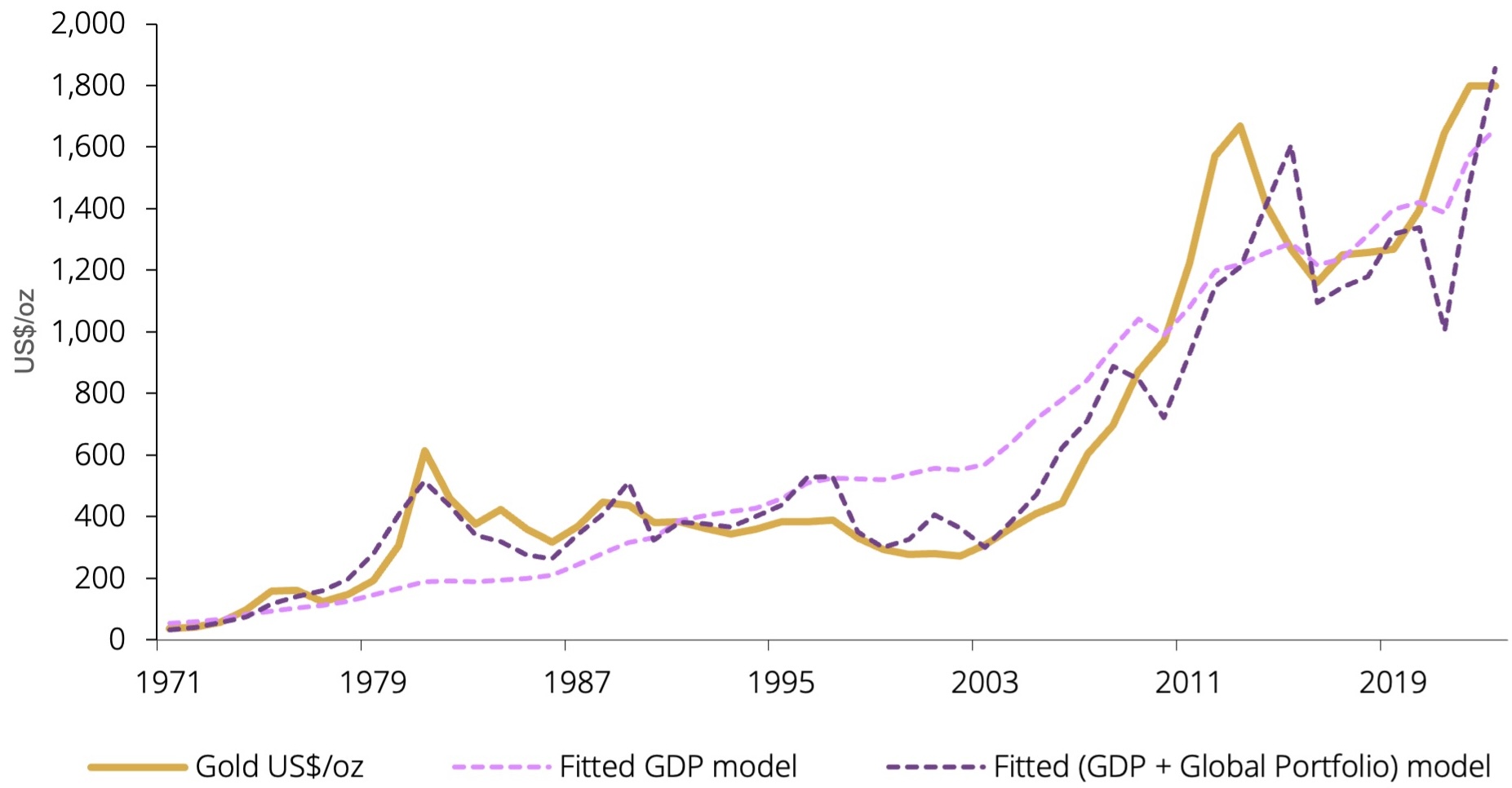
We proxy the economic and financial components using real-world economic and financial variables. Our economic component proxy is global nominal GDP in US dollars. Nominal GDP comprises real GDP, an inflation component (the GDP deflator) and a currency component – used to convert local GDP to US dollars. This captures the flow of capital from income to gold.

Our financial component is proxied using the capitalisation of global equity and bond markets – the global portfolio – in US dollars. It captures the investments available for investors to reallocate income and wealth. It is important to note that we are looking at market capitalisation, accounting for both quantity of float and issuance, not just prices.1

We assess the influence of each of these variables using regression analysis. The analysis reveals that GDP is the primary driver of the gold price in the long run.

The analysis reveals that GDP is the primary driver of the gold price in the long run.

Table 1 presents the regression results for two different specifications. Model (1) is a simple regression to examine the co-movement of gold prices with only GDP. This model yields a positive and statistically significant relationship with 79% (R2) of the variation of gold prices explained by GDP. However, the insignificance of the Phillips-Perron unit-root test result suggests that this simple system does not satisfactorily explain long-run gold prices.

Table 1: Gold’s long run behaviour is explained by global GDP and global portfolio capitalisation

Gold long-term price model (1971-2023)

Dependent variable Log gold price US$/oz
Model (1) Model (2)
Log global nominal GDP 0.821*** 2.837***
Log global portfolio -1.079 **
Observations 53 53
Adjusted R2 79% 92%
Phillips-Perron unit-root test p-value 0.116 0.039***

Note: ***,**,* represent statistical significance at the 1%, 5% and 10% levels respectively. Data from 1971 to 2023.
Source: Bloomberg, BIS, Federal Reserve Bank of St Louis, LBMA Gold Price PM, WFE, World Gold Council. See Appendix A for data descriptions.

Model (2), which we have labelled Gold's Long-Term Expected Return or GLTER, uses both components to create a stable long-run system with an R2 of 92%. A relatively larger coefficient for GDP estimated at 2.8 means that, all else being equal, a 1 unit rise in GDP is associated with a 2.8 unit rise in gold. As we log both sides, these can be interpreted as percentage changes. The negative coefficient for the global portfolio (-1.07) moderates this relationship, as gold is competing for a share of savings, with a one-unit rise in the capitalisation of equity and bond markets associated with a one-unit reduction in gold prices. Once growth as the primary driver of gold prices has been accounted for, we are left with this substitution effect between gold and the global portfolio.

Importantly, the negative coefficient on the global portfolio does not mean that it lowers the price of gold, but that it makes it appreciate at a lower rate.

In this case both the Phillips-Perron test and a Johansen cointegration test2 clearly indicate that there is a long-run relationship and equilibrium between gold prices and the two components.

Once growth as the primary driver of gold prices has been accounted for, we are left with this substitution effect between gold and the global portfolio.

Additional regressions show that individually stocks and bonds each have a negative coefficient when included with GDP in a two-variable system, adding credence to the above finding. See Appendix B for a full discussion.

Chart 2 presents the results of these regressions. The purple dashed line shows the modelled gold price using GDP only, with the errors being particularly pronounced in the 1980s and the 2000s. The graph also displays the fitted line of the full model (black dashed) using both global nominal GDP and the global portfolio capitalisation. The use of two variables rather than one yields a better fit with the price of gold. While it is not surprising that two variables provide a better fit than one, it is notable that the financial variable significantly reduces the deviations from the long-term relationship.

Crucially, using only an economic component to explain gold prices produces a model with rather prolonged periods of disequilibrium (see Table 3 in Appendix B for these results).  Accounting for gold’s dual nature makes for a much more nuanced explanation of gold’s long-run price path.

Chart 2: Gold is influenced by GDP and the global portfolio in the long run

Actual and modelled gold prices*

Footnotes

  1. As such these variables are a composite of prices and issuance. The marginal negative coefficient for bonds in particular may reflect that issuance must often be absorbed regardless of yield, as we saw in Europe after the Global Financial Crisis, which might crowd out investments in alternatives such as gold.

  2. A long-run relationship, or more technically cointegration, implies that two variables co-move in the long run and that any short-run deviation from the long-run path is corrected or reversed.

Important disclaimers and disclosures [+]Important disclaimers and disclosures [-]